California contributors
2016 California Contributors plots
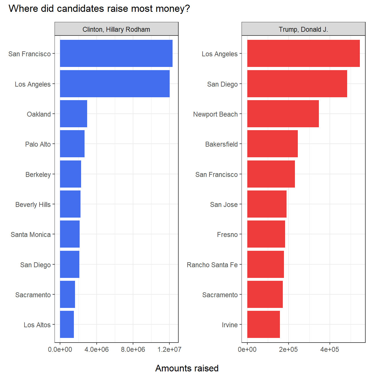
Reproducing the plot that shows the top ten cities in highest amounts raised in political contributions in California during the 2016 US Presidential election.
Merging datasets
# Make sure you use vroom() as it is significantly faster than read.csv()
CA_contributors_2016 <- vroom::vroom(here::here("data","CA_contributors_2016.csv"))

glimpse(CA_contributors_2016)
## Rows: 1,292,843
## Columns: 4
## $ cand_nm <chr> "Clinton, Hillary Rodham", "Clinton, Hillary Rodham"…
## $ contb_receipt_amt <dbl> 50.0, 200.0, 5.0, 48.3, 40.0, 244.3, 35.0, 100.0, 25…
## $ zip <dbl> 94939, 93428, 92337, 95334, 93011, 95826, 90278, 902…
## $ contb_date <date> 2016-04-26, 2016-04-20, 2016-04-02, 2016-11-21, 201…CA_zipcodes <- vroom::vroom(here::here("data","zip_code_database.csv"))
glimpse(CA_zipcodes)## Rows: 42,522
## Columns: 16
## $ zip <chr> "00501", "00544", "00601", "00602", "00603", "006…
## $ type <chr> "UNIQUE", "UNIQUE", "STANDARD", "STANDARD", "STAN…
## $ primary_city <chr> "Holtsville", "Holtsville", "Adjuntas", "Aguada",…
## $ acceptable_cities <chr> NA, NA, NA, NA, "Ramey", "Ramey", NA, NA, NA, NA,…
## $ unacceptable_cities <chr> "I R S Service Center", "Irs Service Center", "Co…
## $ state <chr> "NY", "NY", "PR", "PR", "PR", "PR", "PR", "PR", "…
## $ county <chr> "Suffolk County", "Suffolk County", "Adjuntas", N…
## $ timezone <chr> "America/New_York", "America/New_York", "America/…
## $ area_codes <dbl> 631, 631, 787939, 787, 787, NA, NA, 787939, 787, …
## $ latitude <dbl> 40.8, 40.8, 18.2, 18.4, 18.4, 18.4, 18.4, 18.2, 1…
## $ longitude <dbl> -73.0, -73.0, -66.7, -67.2, -67.2, -67.2, -67.2, …
## $ world_region <chr> NA, NA, NA, NA, NA, NA, NA, NA, NA, NA, NA, NA, N…
## $ country <chr> "US", "US", "US", "US", "US", "US", "US", "US", "…
## $ decommissioned <dbl> 0, 0, 0, 0, 0, 0, 0, 0, 0, 0, 0, 0, 0, 0, 0, 0, 0…
## $ estimated_population <dbl> 384, 0, 0, 0, 0, 0, 0, 0, 0, 0, 0, 0, 0, 0, 0, 0,…
## $ notes <chr> NA, NA, NA, NA, NA, NA, NA, NA, NA, "no NWS data,…#code from the workshop 1 slides
CA_contributors_2016 <- CA_contributors_2016 %>%
mutate(zip = as.character(zip))
CA_contributors_2016 <- left_join(CA_contributors_2016, CA_zipcodes, by="zip")
glimpse(CA_contributors_2016)## Rows: 1,292,843
## Columns: 19
## $ cand_nm <chr> "Clinton, Hillary Rodham", "Clinton, Hillary Rodh…
## $ contb_receipt_amt <dbl> 50.0, 200.0, 5.0, 48.3, 40.0, 244.3, 35.0, 100.0,…
## $ zip <chr> "94939", "93428", "92337", "95334", "93011", "958…
## $ contb_date <date> 2016-04-26, 2016-04-20, 2016-04-02, 2016-11-21, …
## $ type <chr> "STANDARD", "STANDARD", "STANDARD", "STANDARD", "…
## $ primary_city <chr> "Larkspur", "Cambria", "Fontana", "Livingston", "…
## $ acceptable_cities <chr> NA, NA, NA, NA, NA, NA, NA, NA, NA, "Laguna Hills…
## $ unacceptable_cities <chr> NA, NA, NA, NA, NA, "Walsh Station", NA, NA, NA, …
## $ state <chr> "CA", "CA", "CA", "CA", "CA", "CA", "CA", "CA", "…
## $ county <chr> "Marin County", "San Luis Obispo County", "San Be…
## $ timezone <chr> "America/Los_Angeles", "America/Los_Angeles", "Am…
## $ area_codes <dbl> 4.16e+05, 8.05e+02, 9.10e+05, 2.09e+02, 8.05e+02,…
## $ latitude <dbl> 37.9, 35.6, 34.0, 37.3, 34.2, 38.5, 33.9, 33.9, 3…
## $ longitude <dbl> -123, -121, -117, -121, -119, -121, -118, -118, -…
## $ world_region <chr> NA, NA, NA, NA, NA, NA, NA, NA, NA, NA, NA, NA, N…
## $ country <chr> "US", "US", "US", "US", "US", "US", "US", "US", "…
## $ decommissioned <dbl> 0, 0, 0, 0, 0, 0, 0, 0, 0, 0, 0, 0, 0, 0, 0, 0, 0…
## $ estimated_population <dbl> 5652, 5624, 27988, 11811, 1879, 26728, 33427, 334…
## $ notes <chr> NA, NA, NA, NA, NA, NA, NA, NA, NA, "no NWS data,…Transforming data
Hillary <- CA_contributors_2016 %>%
  filter(cand_nm == "Clinton, Hillary Rodham") %>%
  group_by(primary_city, cand_nm) %>%
  summarise(total_contributions = sum(contb_receipt_amt)) %>%
  arrange(desc(total_contributions)) %>%
  head(10)

Hillary_plot <- ggplot(Hillary,
       aes(x = total_contributions,
           y = fct_reorder(primary_city, total_contributions))) +
  geom_bar(stat='identity', fill = "royalblue2") +
  labs(
    y = NULL,
    x = NULL,
  ) +
  theme_bw() +
  theme(legend.position="none") +
  facet_wrap(~ cand_nm)

Donald <- CA_contributors_2016 %>%
  filter(cand_nm == "Trump, Donald J.") %>%
  group_by(primary_city, cand_nm) %>%
  summarise(total_contributions = sum(contb_receipt_amt)) %>%
  arrange(desc(total_contributions)) %>%
  head(10)

Donald_plot <- ggplot(Donald,
       aes(x = total_contributions,
           y = fct_reorder(primary_city, total_contributions))) +
  geom_bar(stat='identity', fill = "brown2") +
  labs(
    y = NULL,
    x = NULL,
  ) +
  theme_bw() +
  theme(legend.position="none") +
  facet_wrap(~ cand_nm)
Joining plots together
library(patchwork)

plots <- Hillary_plot + Donald_plot + plot_annotation(title = "Where did candidates raise most money?") + plot_layout(widths = 2000)  #joining two plots using patchwork package


# code taken from https://github.com/thomasp85/patchwork/issues/150 to add label on the x-axis between two plots
gt <- patchwork::patchworkGrob(plots)
gridExtra::grid.arrange(gt, bottom = "Amounts raised")